
swift_too module
Swift_ObsQuery example - querying past Swift observations
API version = 1.2, swifttools version = 2.4
Author: Jamie A. Kennea (Penn State)
The Swift_ObsQuery class allows for querying the database of observations have have already been performed by Swift, otherwise known as the "As-Flown Science Timeline" (AFST). Note this will only fetch observations that have already been performed, not scheduled observations.
%matplotlib inline
import matplotlib.pyplot as plt
from swifttools.swift_too import ObsQuery
from time import sleep
import numpy as np
Constructing the query
Note: As of swifttools version 2.2, you do not need to pass username or shared_secret keywords, they will default to anonymous. This is the recommended usage for anything except a TOO request.
First example, how often has Swift observed the binary system SS 433? Well, I can't remember the RA/Dec off the top of my head, so let's look it up...
New features in swifttools 2.3
swifttools 2.3 supports a new class called Swift_Resolve. You can use this to do name resolution, i.e. converting the name of a target into coordinates. However, it's also built into classes that take RA/Dec now, so you can just pass it using the name parameters.
Another new feature of 2.3, there are now shorthand names for classes, so you can omit the Swift_ when calling the class, changing it to just ObsQuery.
query = ObsQuery()
query.name = "SS 433"
Now you can see the coordinates, as either RA/Dec or astropy's SkyCoord, using the attributes ra, dec and skycoord (if astropy is installed). For example:
query.skycoord<SkyCoord (FK5: equinox=J2000.000): (ra, dec) in deg
(287.95651875, 4.98272889)>RA/Dec is stored by the TOO API in decimal degrees, in J2000 epoch as this is the epoch Swift uses
print(f"RA/Dec(J2000) = {query.ra:.4f}, {query.dec:.4f}")RA/Dec(J2000) = 287.9565, 4.9827Looks legit. However, we can also set RA/Dec the old fashioned way
query.ra, query.dec = 287.9565, 4.9827Note that skycoord will remain correct even if you changed the ra and dec properties.
query.skycoord<SkyCoord (FK5: equinox=J2000.000): (ra, dec) in deg
(287.9565, 4.9827)>Swift_ObsQuery has a default search radius which is....
print(f"Default search radius = {query.radius:.3f} degrees")Default search radius = 0.197 degreesThat's 12 arcminutes, which is the approximate field of view of Swift's X-ray Telescope (XRT). We can narrow that down a bit, so we only get matches that are in the center of the field of view (FOV), and also in UVOT which has a smaller FOV.
query.radius = 5 / 60 # 5 arc-minutes, as the units for radius are degreesSubmitting the query
OK let's query the Swift timeline to see how many observations it's taken. This might take a few seconds to process. query method will return True if everything is OK, False if there is a problem. If there is a problem, simply look at the contents of the status attribute.
if query.submit():
    print("Success!")
else:
print(f"Fail or timeout? {query.status}")Success!Looks like that worked, let's take a look at the status attribute anyway.
query.status| Parameter | Value |
|---|---|
| username | anonymous |
| jobnumber | 281226 |
| status | Accepted |
Examining the results of the query
So how many observations has Swift taken of this target?
print(f"This many: {len(query)}")This many: 77That's a lot of damage. Here's a thing to remember, every entry in this is a single snapshot of observation. As Swift is in a low Earth orbit, it means that a snapshot is typically max 30 mins, or sometimes a bit longer (~44 mins), so a long exposure will consist of multiple snapshots. Observations are grouped by obsid (a 12 digit number with leading zeros), so snapshots with the same obsid are part of the same planned observation.
query| Begin Time | End Time | Target Name | Observation Number | Exposure (s) | Slewtime (s) |
|---|---|---|---|---|---|
| 2005-07-30 13:23:02 | 2005-07-30 13:27:00 | SS433 | 00035190001 | 95 | 143 |
| 2005-07-30 13:27:02 | 2005-07-30 13:30:48 | SS433 | 00035190002 | 210 | 16 |
| 2005-08-01 13:36:02 | 2005-08-01 13:40:00 | SS433 | 00035190005 | 95 | 143 |
| 2005-08-01 13:40:02 | 2005-08-01 13:56:58 | SS433 | 00035190006 | 1000 | 16 |
| 2005-08-01 18:44:15 | 2005-08-01 18:46:32 | SS433 | 00035190007 | 0 | 137 |
| 2005-08-01 18:46:35 | 2005-08-01 19:08:01 | SS433 | 00035190008 | 1270 | 16 |
| 2005-08-18 00:59:02 | 2005-08-18 01:14:58 | SS433 | 00035190013 | 870 | 86 |
| 2005-08-18 02:35:02 | 2005-08-18 02:51:58 | SS433 | 00035190013 | 930 | 86 |
| 2006-06-30 13:45:02 | 2006-06-30 13:55:00 | SS 433 | 00035190014 | 425 | 173 |
| 2006-06-30 15:19:02 | 2006-06-30 15:31:00 | SS 433 | 00035190014 | 545 | 173 |
| 2006-06-30 16:56:02 | 2006-06-30 17:08:00 | SS 433 | 00035190014 | 545 | 173 |
| 2006-06-30 18:32:02 | 2006-06-30 18:44:00 | SS 433 | 00035190014 | 545 | 173 |
| 2006-06-30 20:09:02 | 2006-06-30 20:21:00 | SS 433 | 00035190014 | 545 | 173 |
| 2006-06-30 21:45:01 | 2006-06-30 21:57:00 | SS 433 | 00035190014 | 545 | 174 |
| 2006-06-30 23:22:02 | 2006-06-30 23:27:00 | SS 433 | 00035190014 | 125 | 173 |
| 2006-07-01 02:34:02 | 2006-07-01 02:43:56 | SS 433 | 00035190015 | 435 | 159 |
| 2006-07-01 04:11:02 | 2006-07-01 04:24:56 | SS 433 | 00035190015 | 675 | 159 |
| 2006-07-01 05:47:02 | 2006-07-01 05:59:01 | SS 433 | 00035190015 | 560 | 159 |
| 2006-07-01 07:24:02 | 2006-07-01 07:34:58 | SS 433 | 00035190015 | 485 | 171 |
| 2006-07-01 09:00:02 | 2006-07-01 09:11:57 | SS 433 | 00035190015 | 535 | 180 |
| 2006-07-01 10:36:02 | 2006-07-01 10:47:57 | SS 433 | 00035190015 | 535 | 180 |
| 2006-07-01 12:13:02 | 2006-07-01 12:23:58 | SS 433 | 00035190015 | 485 | 171 |
| 2006-07-01 20:15:02 | 2006-07-01 20:25:58 | SS 433 | 00035190015 | 475 | 181 |
| 2006-07-01 21:51:02 | 2006-07-01 22:02:57 | SS 433 | 00035190015 | 535 | 180 |
| 2006-07-02 02:41:02 | 2006-07-02 02:50:58 | SS 433 | 00035190015 | 415 | 181 |
| 2006-07-02 04:17:02 | 2006-07-02 04:31:57 | SS 433 | 00035190015 | 715 | 180 |
| 2006-07-02 05:53:02 | 2006-07-02 06:04:57 | SS 433 | 00035190015 | 540 | 175 |
| 2006-07-02 07:30:02 | 2006-07-02 07:40:57 | SS 433 | 00035190015 | 480 | 175 |
| 2006-07-02 09:06:02 | 2006-07-02 09:16:57 | SS 433 | 00035190015 | 480 | 175 |
| 2006-07-02 10:43:02 | 2006-07-02 10:53:56 | SS 433 | 00035190015 | 480 | 174 |
| 2006-11-03 18:42:58 | 2006-11-03 18:46:57 | SS433 | 00035190016 | 20 | 219 |
| 2006-11-03 19:06:02 | 2006-11-03 19:28:25 | SS433 | 00035190016 | 1285 | 58 |
| 2006-11-03 20:19:35 | 2006-11-03 21:04:35 | SS433 | 00035190016 | 2481 | 219 |
| 2006-11-03 21:55:59 | 2006-11-03 22:20:08 | SS433 | 00035190016 | 1230 | 219 |
| 2007-09-12 13:31:01 | 2007-09-12 13:45:59 | SS433 | 00035190020 | 785 | 113 |
| 2007-09-13 13:37:01 | 2007-09-13 13:47:58 | SS433 | 00035190021 | 535 | 122 |
| 2007-09-14 13:37:01 | 2007-09-14 13:52:00 | SS433 | 00035190022 | 790 | 109 |
| 2007-09-15 01:02:01 | 2007-09-15 01:15:56 | SS433 | 00035190023 | 785 | 50 |
| 2007-09-16 17:11:01 | 2007-09-16 17:23:57 | SS433 | 00035190023 | 725 | 51 |
| 2007-09-27 21:17:01 | 2007-09-27 21:34:58 | SS433 | 00035190025 | 995 | 82 |
| 2012-10-15 23:45:20 | 2012-10-16 00:03:22 | SS433 | 00035190026 | 1000 | 82 |
| 2014-07-28 14:26:50 | 2014-07-28 14:32:27 | SS433 | 00035190027 | 185 | 152 |
| 2014-07-28 15:24:35 | 2014-07-28 15:56:23 | SS433 | 00035190027 | 1810 | 98 |
| 2014-09-26 07:20:47 | 2014-09-26 07:25:58 | SS433 | 00035190028 | 185 | 126 |
| 2014-09-26 08:33:02 | 2014-09-26 08:45:57 | SS433 | 00035190028 | 655 | 120 |
| 2014-09-26 10:14:02 | 2014-09-26 10:18:32 | SS433 | 00035190028 | 150 | 120 |
| 2014-10-01 18:00:02 | 2014-10-01 18:14:00 | SS433 | 00035190030 | 745 | 93 |
| 2014-10-03 13:10:02 | 2014-10-03 13:26:59 | SS433 | 00035190031 | 845 | 172 |
| 2014-10-04 03:33:02 | 2014-10-04 03:46:57 | SS433 | 00080803001 | 740 | 95 |
| 2014-10-04 08:18:02 | 2014-10-04 08:34:57 | SS433 | 00080803001 | 865 | 150 |
| 2014-10-04 13:07:02 | 2014-10-04 13:16:57 | SS433 | 00080803001 | 490 | 105 |
| 2014-10-05 13:18:09 | 2014-10-05 13:33:57 | SS433 | 00035190032 | 880 | 68 |
| 2014-10-07 00:24:02 | 2014-10-07 00:40:59 | SS433 | 00035190033 | 870 | 147 |
| 2014-10-09 00:12:02 | 2014-10-09 00:28:59 | SS433 | 00035190034 | 935 | 82 |
| 2014-10-17 04:47:02 | 2014-10-17 04:59:57 | SS433 | 00080803002 | 655 | 120 |
| 2014-10-17 06:34:02 | 2014-10-17 06:52:41 | SS433 | 00080803002 | 1015 | 104 |
| 2014-10-17 14:52:02 | 2014-10-17 15:02:57 | SS433 | 00080803002 | 510 | 145 |
| 2014-10-30 16:06:02 | 2014-10-30 16:24:58 | SS433 | 00080803003 | 1070 | 66 |
| 2014-10-30 17:46:02 | 2014-10-30 18:00:58 | SS433 | 00080803003 | 830 | 66 |
| 2014-11-12 20:14:02 | 2014-11-12 20:35:59 | SS433 | 00080803004 | 1170 | 147 |
| 2014-11-12 21:50:02 | 2014-11-12 22:08:59 | SS433 | 00080803004 | 960 | 177 |
| 2014-11-25 11:56:02 | 2014-11-25 12:25:58 | SS433 | 00080803005 | 1585 | 211 |
| 2014-11-25 13:32:02 | 2014-11-25 13:41:58 | SS433 | 00080803005 | 445 | 151 |
| 2015-02-24 23:17:02 | 2015-02-24 23:46:58 | SS433 | 00080803006 | 1655 | 141 |
| 2015-03-11 05:28:01 | 2015-03-11 05:47:00 | SS433 | 00080803008 | 1055 | 84 |
| 2015-03-11 07:05:02 | 2015-03-11 07:21:59 | SS433 | 00080803008 | 925 | 92 |
| 2015-03-23 22:11:02 | 2015-03-23 22:29:57 | SS433 | 00080803009 | 1055 | 80 |
| 2015-03-23 23:44:02 | 2015-03-23 23:59:56 | SS433 | 00080803009 | 875 | 79 |
| 2015-04-18 19:22:02 | 2015-04-18 19:51:57 | SS433 | 00080803010 | 1675 | 120 |
| 2015-04-18 21:07:10 | 2015-04-18 21:10:29 | SS433 | 00080803010 | 0 | 199 |
| 2015-06-22 22:47:02 | 2015-06-22 23:06:59 | SS433 | 00035190035 | 1135 | 62 |
| 2015-07-05 08:54:02 | 2015-07-05 08:55:50 | SS433 | 00080803011 | 15 | 93 |
| 2015-07-05 10:49:02 | 2015-07-05 11:09:59 | SS433 | 00080803011 | 1205 | 52 |
| 2018-07-25 07:17:02 | 2018-07-25 07:24:59 | SS433 | 00035190036 | 355 | 122 |
| 2018-07-25 16:48:02 | 2018-07-25 17:00:58 | SS433 | 00035190036 | 680 | 96 |
| 2018-08-29 10:43:02 | 2018-08-29 10:50:59 | SS433 | 00035190037 | 395 | 82 |
| 2018-08-29 23:31:01 | 2018-08-29 23:45:57 | SS433 | 00035190037 | 805 | 91 |
Wow that is a lot of observations.
Pointing Accuracy
Here's an interesting thing about Swift, it doesn't point very accurately. This is because the ACS system sacrifices accuracy for speed. The goal is to get the object of interest into the field of view of XRT and UVOT, not at the boresight. As a result, the pointing direction be typically up to 3 arcminutes off the requested pointing direction. Note that for each entry listed above, we give an ra and dec value, so let's check out the variation:
plt.figure()
plt.plot(
    [float(entry.ra) for entry in query], [float(entry.dec) for entry in query], "+"
)
plt.plot(
    [entry.ra_object for entry in query], [entry.dec_object for entry in query], "X"
)
plt.xlabel("RA(J2000)")
plt.ylabel("Dec(J2000)")
_ = plt.title(f"{query.name} pointing scatter")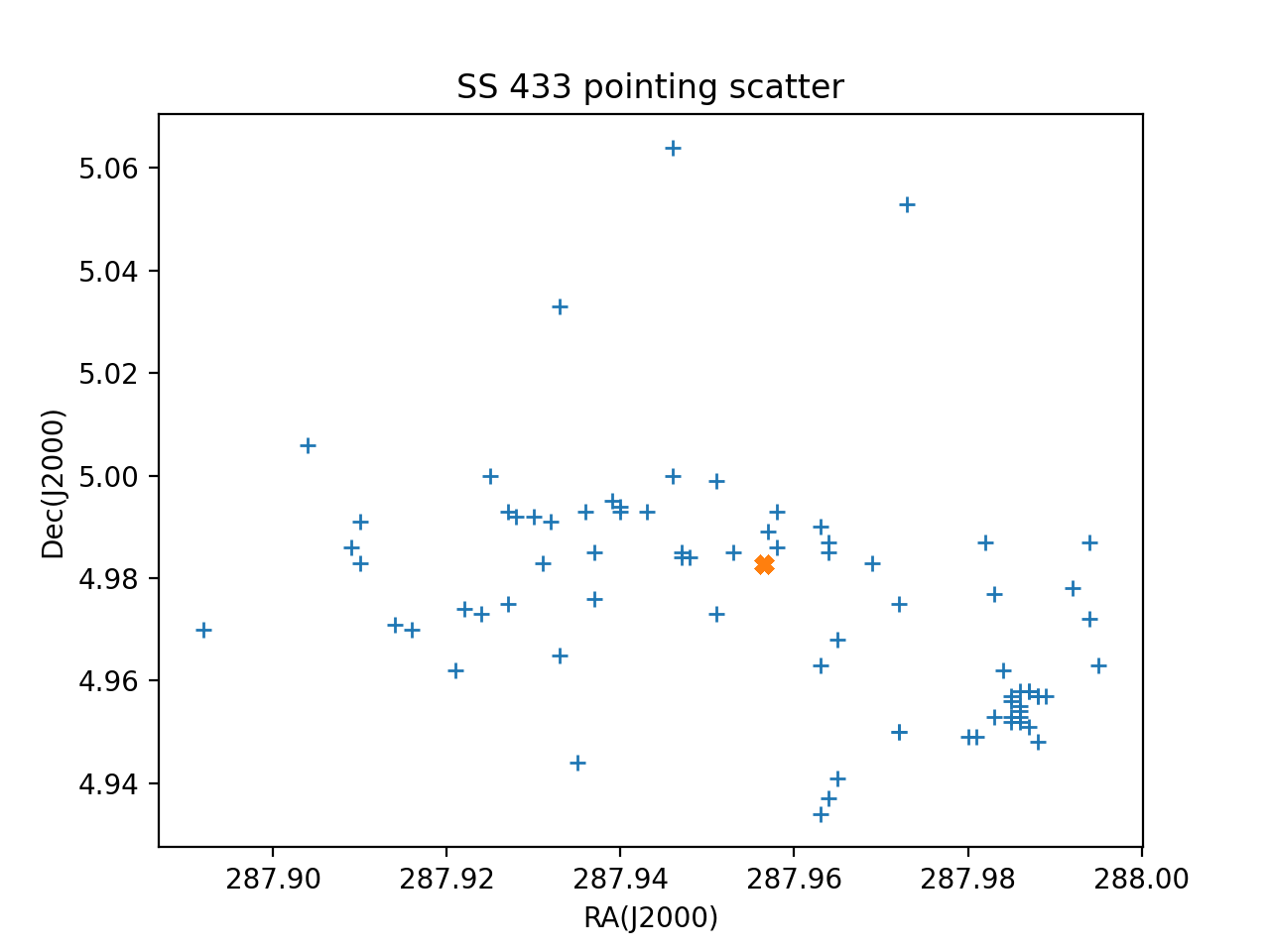
As you can see there's a lot of variation of the pointing direction. Each entry also has a values ra_object, dec_object, which give the decimal degrees values of the requested pointing direction for each observation. This typically will be the coordinates of the Target of the Observation, but sometimes if offsets are applied for any reason, it might differ.
The ra_object/dec_object values aren't necessarily going to be for the object you queried on. In fact there can be multiple values of ra_point/dec_point if the queried field lies inside multiple pointings.
Although the RA/Dec are returned in J2000 decimal degrees, they're also returned as skycoords. However, ra_object and dec_object are not so we will have to convert those to SkyCoords manually.
query[0].skycoord<SkyCoord (FK5: equinox=J2000.000): (ra, dec) in deg
(287.994, 4.972)>Sometimes ra_object, dec_object cannot be determined, so the value will be 'None'. I'm going to filter those out so we can do some comparing.
from astropy.coordinates import SkyCoord
import astropy.units as u

sc = SkyCoord([entry.skycoord for entry in query if entry.ra_point != None])
scp = SkyCoord(
    [entry.ra_point for entry in query if entry.ra_point != None],
    [entry.dec_point for entry in query if entry.ra_point != None],
    frame="fk5",
    unit=(u.deg, u.deg),
)
I made an array of ra_point/dec_point so we can evaluate how accurately Swift actually pointed at this target. Let's make a histogram of the pointing offsets.
plt.figure()
plt.hist(sc.separation(scp).arcmin, bins=30)
plt.ylabel("Number of pointings")
plt.xlabel("Offset from requested pointing direction (arc-minutes)")
print(f"Median offset value = {np.median(sc.separation(scp).arcmin):0.2f} arc-minutes")
Median offset value = 2.17 arc-minutes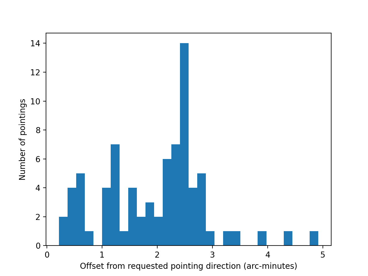
So you'll see that the median offset here is around 2 arc-minutes, with a pretty big scatter, and there may even be some large outliers.
Grouping Snapshots into Observations
Let's take a look at an individual entry to see what information is being returned by this query.
query[0]| Begin Time | End Time | Target Name | Observation Number | Exposure (s) | Slewtime (s) |
|---|---|---|---|---|---|
| 2005-07-30 13:23:02 | 2005-07-30 13:27:00 | SS433 | 00035190001 | 95 | 143 |
So some useful information here. Firstly remember each entry represents a snapshot of Swift data, that is data taken in a single orbit of observations. Typically data that you obtain from the SDC will be grouped by observation, and those observations can contain many snapshots. Observations have a unique target ID (target ID) and segment (seg) numbers. These typically are combined into a Observation Number (obsnum), which in the SDC format will look like a concatibation of the target ID, and segment, with padding zeros, e.g.:
print(
    f"Target ID = {query[0].targetid}, segment = {query[0].seg}, ObservationID = {query[0].obsnum}"
)
Target ID = 35190, segment = 1, ObservationID = 00035190001If you're interested in all the observations under a particular Observation ID, then there's a property called "observations" that contains a dictionary of all observations on an Observation ID basis. Let's look at the summary of this dictionary by just printing out all the entries.
query.observations| Begin Time | End Time | Target Name | Observation Number | Exposure (s) | Slewtime (s) |
|---|---|---|---|---|---|
| 2005-07-30 13:23:02 | 2005-07-30 13:27:00 | SS433 | 00035190001 | 95 | 143 |
| 2005-07-30 13:27:02 | 2005-07-30 13:30:48 | SS433 | 00035190002 | 210 | 16 |
| 2005-08-01 13:36:02 | 2005-08-01 13:40:00 | SS433 | 00035190005 | 95 | 143 |
| 2005-08-01 13:40:02 | 2005-08-01 13:56:58 | SS433 | 00035190006 | 1000 | 16 |
| 2005-08-01 18:44:15 | 2005-08-01 18:46:32 | SS433 | 00035190007 | 0 | 137 |
| 2005-08-01 18:46:35 | 2005-08-01 19:08:01 | SS433 | 00035190008 | 1270 | 16 |
| 2005-08-18 00:59:02 | 2005-08-18 02:51:58 | SS433 | 00035190013 | 1800 | 172 |
| 2006-06-30 13:45:02 | 2006-06-30 23:27:00 | SS 433 | 00035190014 | 3275 | 1212 |
| 2006-07-01 02:34:02 | 2006-07-02 10:53:56 | SS 433 | 00035190015 | 7830 | 2600 |
| 2006-11-03 18:42:58 | 2006-11-03 22:20:08 | SS433 | 00035190016 | 5016 | 715 |
| 2007-09-12 13:31:01 | 2007-09-12 13:45:59 | SS433 | 00035190020 | 785 | 113 |
| 2007-09-13 13:37:01 | 2007-09-13 13:47:58 | SS433 | 00035190021 | 535 | 122 |
| 2007-09-14 13:37:01 | 2007-09-14 13:52:00 | SS433 | 00035190022 | 790 | 109 |
| 2007-09-15 01:02:01 | 2007-09-16 17:23:57 | SS433 | 00035190023 | 1510 | 101 |
| 2007-09-27 21:17:01 | 2007-09-27 21:34:58 | SS433 | 00035190025 | 995 | 82 |
| 2012-10-15 23:45:20 | 2012-10-16 00:03:22 | SS433 | 00035190026 | 1000 | 82 |
| 2014-07-28 14:26:50 | 2014-07-28 15:56:23 | SS433 | 00035190027 | 1995 | 250 |
| 2014-09-26 07:20:47 | 2014-09-26 10:18:32 | SS433 | 00035190028 | 990 | 366 |
| 2014-10-01 18:00:02 | 2014-10-01 18:14:00 | SS433 | 00035190030 | 745 | 93 |
| 2014-10-03 13:10:02 | 2014-10-03 13:26:59 | SS433 | 00035190031 | 845 | 172 |
| 2014-10-04 03:33:02 | 2014-10-04 13:16:57 | SS433 | 00080803001 | 2095 | 350 |
| 2014-10-05 13:18:09 | 2014-10-05 13:33:57 | SS433 | 00035190032 | 880 | 68 |
| 2014-10-07 00:24:02 | 2014-10-07 00:40:59 | SS433 | 00035190033 | 870 | 147 |
| 2014-10-09 00:12:02 | 2014-10-09 00:28:59 | SS433 | 00035190034 | 935 | 82 |
| 2014-10-17 04:47:02 | 2014-10-17 15:02:57 | SS433 | 00080803002 | 2180 | 369 |
| 2014-10-30 16:06:02 | 2014-10-30 18:00:58 | SS433 | 00080803003 | 1900 | 132 |
| 2014-11-12 20:14:02 | 2014-11-12 22:08:59 | SS433 | 00080803004 | 2130 | 324 |
| 2014-11-25 11:56:02 | 2014-11-25 13:41:58 | SS433 | 00080803005 | 2030 | 362 |
| 2015-02-24 23:17:02 | 2015-02-24 23:46:58 | SS433 | 00080803006 | 1655 | 141 |
| 2015-03-11 05:28:01 | 2015-03-11 07:21:59 | SS433 | 00080803008 | 1980 | 176 |
| 2015-03-23 22:11:02 | 2015-03-23 23:59:56 | SS433 | 00080803009 | 1930 | 159 |
| 2015-04-18 19:22:02 | 2015-04-18 21:10:29 | SS433 | 00080803010 | 1675 | 319 |
| 2015-06-22 22:47:02 | 2015-06-22 23:06:59 | SS433 | 00035190035 | 1135 | 62 |
| 2015-07-05 08:54:02 | 2015-07-05 11:09:59 | SS433 | 00080803011 | 1220 | 145 |
| 2018-07-25 07:17:02 | 2018-07-25 17:00:58 | SS433 | 00035190036 | 1035 | 218 |
| 2018-08-29 10:43:02 | 2018-08-29 23:45:57 | SS433 | 00035190037 | 1200 | 173 |
You can see that now the summary shows the details for an entire observation, with the begin and end times being those of associated with the first and last observation of that Observation ID, and the exposure time being the total. Importantly due to orbit gaps, the exposure time is not just end minus begin. Each entry in the observations dictionary contains details on the individual segments also. Note that Observation ID is a string, given as it is formatted with padding zeros. For example:
query.observations["00035190015"]| Begin Time | End Time | Target Name | Observation Number | Exposure (s) | Slewtime (s) |
|---|---|---|---|---|---|
| 2006-07-01 02:34:02 | 2006-07-02 10:53:56 | SS 433 | 00035190015 | 7830 | 2600 |
If we want to see what snapshots make up a particular observation, it's easy:
query.observations["00035190015"].snapshots| Begin Time | End Time | Target Name | Observation Number | Exposure (s) | Slewtime (s) |
|---|---|---|---|---|---|
| 2006-07-01 02:34:02 | 2006-07-01 02:43:56 | SS 433 | 00035190015 | 435 | 159 |
| 2006-07-01 04:11:02 | 2006-07-01 04:24:56 | SS 433 | 00035190015 | 675 | 159 |
| 2006-07-01 05:47:02 | 2006-07-01 05:59:01 | SS 433 | 00035190015 | 560 | 159 |
| 2006-07-01 07:24:02 | 2006-07-01 07:34:58 | SS 433 | 00035190015 | 485 | 171 |
| 2006-07-01 09:00:02 | 2006-07-01 09:11:57 | SS 433 | 00035190015 | 535 | 180 |
| 2006-07-01 10:36:02 | 2006-07-01 10:47:57 | SS 433 | 00035190015 | 535 | 180 |
| 2006-07-01 12:13:02 | 2006-07-01 12:23:58 | SS 433 | 00035190015 | 485 | 171 |
| 2006-07-01 20:15:02 | 2006-07-01 20:25:58 | SS 433 | 00035190015 | 475 | 181 |
| 2006-07-01 21:51:02 | 2006-07-01 22:02:57 | SS 433 | 00035190015 | 535 | 180 |
| 2006-07-02 02:41:02 | 2006-07-02 02:50:58 | SS 433 | 00035190015 | 415 | 181 |
| 2006-07-02 04:17:02 | 2006-07-02 04:31:57 | SS 433 | 00035190015 | 715 | 180 |
| 2006-07-02 05:53:02 | 2006-07-02 06:04:57 | SS 433 | 00035190015 | 540 | 175 |
| 2006-07-02 07:30:02 | 2006-07-02 07:40:57 | SS 433 | 00035190015 | 480 | 175 |
| 2006-07-02 09:06:02 | 2006-07-02 09:16:57 | SS 433 | 00035190015 | 480 | 175 |
| 2006-07-02 10:43:02 | 2006-07-02 10:53:56 | SS 433 | 00035190015 | 480 | 174 |
You can query the exposure and other infomation for the combined snapshots in the Observation ID.
query.observations["00035190015"].exposuredatetime.timedelta(seconds=7830)Note that the result here is a datetime timedelta object. You can easily get the seconds as an integer or convert to an astropy TimeDelta object.
query.observations["00035190015"].exposure.seconds7830from astropy.time import TimeDelta
TimeDelta(query.observations["00035190015"].exposure)<TimeDelta object: scale='None' format='datetime' value=2:10:30>Note that there is no RA/Dec (ra/dec) for an observation, only the requested pointing direction (ra_point/dec_point), because actual RA/Dec will be different for each snapshot, so delve into the individual snapshots for those.
query.observations["00035190015"].ra_point, query.observations["00035190015"].dec_point(287.9565, 4.982667)Instrument Configuration
All observations for a given Observation ID will have the same instrument configuration. Let's check those out.
print(
    f"XRT mode = {query.observations['00035190015'].xrt}, UVOT mode = {query.observations['00035190015'].uvot}"
)
XRT mode = Auto, UVOT mode = 0x20edIn this case the XRT mode is Auto, which means that XRT itself decides whether to be in PC or WT mode, based on the brightness of sources in the central 200x200 pixels of the detector, roughly the central 8.5 arcmin x 8.5 arcmin box. Because of this we can't determine what mode XRT will have actually taken the data in without looking at it. However for many observation, the mode is fixed, here you will see results like so:
print(f"XRT mode = {query.observations['00035190037'].xrt}")XRT mode = PCAs this is PC mode, we can guarantee that the data are taken in PC mode.
For UVOT the mode above is a hex number 0x20ed. There are a large number of modes that can be used with UVOT, given it's many different combinations of filters, exposure windows, etc. Luckily you can query what this mode means using the UVOT_mode class. We can quickly display a table showing details of the mode as follows:
from swifttools.swift_too import UVOT_mode

UVOT_mode(uvotmode=query.observations["00035190015"].uvot)
UVOT Mode: 0x20ed
Swift Mission Operations Center
The Pennsylvania State University301 Science Park Road,
Building 2 Suite 332,
State College, PA 16801
USA
☎ +1 (814) 865-6834
📧 swiftods@swift.psu.edu
Swift MOC Team Leads
Mission Director: John NousekScience Operations: Jamie Kennea
Flight Operations: Mark Hilliard
UVOT: Michael Siegel
XRT: Jamie Kennea
Swift Partners
UK: UCL MSSL Univ. of LeicesterUSA: NASA/GSFC LANL Omitron SwRI
Italy: SSDC/ASI INAF OA-Brera